CUPED and Variants: A/B Tests in Half the Time
CUPED, CUPAC, MLRATE. The variance reduction package running on every modern A/B platform
How Microsoft, DoorDash and Meta cut A/B test time in half using data they already had, and why the metric matters more than the technique
In the previous article I mentioned CUPED in passing as “a technique that reduces sample size without changing the methodology”. That came out way too short for what this thing actually does.
CUPED (Controlled-experiment Using Pre-Experiment Data) was published in 2013 by Deng, Xu, Kohavi and Walker, at Microsoft. The original paper shows that, using pre-experiment behavior as a covariate, they managed to reduce the variance of Bing’s metrics by about 50%. 50% less variance means half the sample size to detect the same effect, in other words, half the time. For a company running thousands of A/B tests a year, that is doubling iteration speed without touching anything visible in the product.
Today CUPED is implemented in the internal platforms of Microsoft, Netflix, Booking, Airbnb, Meta, Uber, DoorDash, Etsy, Faire, TripAdvisor, and in every major commercial platform, Statsig, Eppo, VWO, Kameleoon, Amplitude. If you run A/B tests on anything modern, CUPED is probably already running under the hood without you seeing it.
The structure of this article goes like this. First classic CUPED (intuition, math, why it works), then the two modern extensions, DoorDash’s CUPAC (2020) and Meta’s MLRATE (2021). Next I cover where the thing can break, and I close with a broad guide on how to think about adopting it in your experimentation program.
The intuition, heavy users were already heavy before the test
Picture any platform with the metric “sessions per user in 14 days”. The power of your test is a function of the variance of that metric, and the variance is high because users are very heterogeneous. Some users open the app 80 times a week, some open it twice a month. When you compare control and treatment, a big part of the noise is simply that difference between user types randomly landing in each group.
Randomization takes care of that on average, but in any given sample there will always be some leftover difference, and that residual difference is what inflates your confidence interval and asks for more N.
The observation that changes the approach: today’s heavy user is the heavy user from 30 days ago. If I know user X did 80 sessions in the 30 days before the experiment, I can predict, with no sophisticated model, that they will do more sessions than average during the experiment. The prediction has nothing to do with the treatment effect. What I am predicting is their baseline.
The CUPED idea is simple. Instead of comparing Y_treatment with Y_control, I compare Y_treatment - baseline_prediction with Y_control - baseline_prediction. The baseline heterogeneity goes away, and the only thing left is the treatment effect (which is what I wanted from the start) plus a smaller residual noise.
It invents no information. It only removes a chunk of variance you already knew existed and that has nothing to do with what is being tested.
The math
The CUPED adjustment is one line:
Y_cuped = Y - theta * (X - mean(X))where:
- Y is the metric during the experiment (e.g. sessions in 14 days)
- X is the pre-experiment metric (e.g. sessions in the previous 30 days)
- theta = cov(Y, X) / var(X) is the coefficient that minimizes the residual variance
That is a linear regression of Y on X. Theta is the slope of the line that best predicts Y from X.
The variance of Y_cuped is, in the limit:
var(Y_cuped) ≈ var(Y) * (1 - rho²)where rho is the correlation between Y and X. The higher the correlation between pre and during behavior, the bigger the reduction. Nothing beyond that.
In short, a table:
 rho  |  var reduction  |  equivalent sample size
------+-----------------+-------------------------
 0.3  |        9%       |  91% of the original N
 0.5  |       25%       |  75% of the original N
 0.7  |       49%       |  51% of the original N
 0.8  |       64%       |  36% of the original N
 0.9  |       81%       |  19% of the original N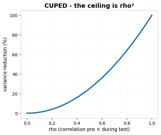
Variance reduction as a function of rho. CUPED delivers exactly rho² of the original variance, no more, no less. Microsoft saw ~50% on Bing because rho there sits between 0.7 and 0.8.
Microsoft cites typical rho between 0.6 and 0.8 on Bing’s metrics, which gives variance reductions of 36% to 64%, in line with the 50% they reported. The difference between a platform that adopts CUPED and gains 50% and one that adopts it and gains 5% is rho, and rho is a function of the metric. The technique plays no part in it.
Why this introduces no bias
The natural question is, “if I mess with Y, won’t I bias the test?”.
No, and the reason is structural. X is pre-experiment. It was observed before the treatment was applied. By construction, X is independent of T (the treatment indicator). Since theta * (X - mean(X)) has mean zero and does not depend on T, subtracting it from Y does not change the difference between groups.
In formula:
E[Y_cuped | T=1] - E[Y_cuped | T=0] = E[Y | T=1] - E[Y | T=0]The mean of the difference is the same. What changes is the variance. The noise between individuals drops, so the standard error of the difference drops with it, so the p-value drops (when there is an effect) and the confidence interval gets narrower.
One detail. Theta has to be estimated on the whole pool (control + treatment), never separately per group. Estimating per group introduces bias because theta starts capturing part of the treatment effect.
This property deserves a highlight. Several A/B “optimizations” seem to increase power but are actually just inflating false positives (peeking, p-hacking, ad-hoc segmentation, all mentioned in the previous article). CUPED is mathematically unbiased. It narrows the confidence interval without moving the center.
CUPAC, DoorDash’s extension (2020), ML as the covariate
Classic CUPED uses one covariate (X) at a time. But in production, you almost always have several pre-experiment features: recency, historical spend, session count, favorite category, device, location, acquisition channel. Combining all of that by hand is laborious and rarely optimal.
In 2020, Jeff Li, Yixin Tang and Jared Bauman at DoorDash published a blog post describing CUPAC, Control Using Predictions As Covariate. The idea is a clean generalization:
- Train an ML model (GBM, random forest, neural net) to predict Y from all available pre-experiment features.
- Use the model’s prediction as CUPED’s “X”.
Why is that better than classic CUPED? Because an ML model captures non-linear relationships and interactions between features that a single covariate cannot. If “new user + high pre spend + category X” predicts during-experiment behavior better than each one in isolation, the model learns that, and the variance reduction grows.
Modern CUPAC is cross-fitted, the standard today at DoorDash (Dash-AB, 2022) and Etsy (2025). The idea is to train the model on K folds (usually 5), producing out-of-sample predictions for every user. That avoids two problems:
- Leakage. If you train on the whole pool, the model learns individual noise and part of the treatment effect.
- Too small. If you train only on the control group, you lose half the sample size, and the model predicts out of distribution on treatment.
Cross-fitting solves both. Every user is predicted by a model trained on other users. Without it, CUPAC can actually make variance worse instead of better.
At DoorDash, in logistics systems with switchback testing, CUPAC delivered about 10% more variance reduction than plain CUPED. Etsy reported in 2025 that moving from CUPED to CUPAC shortened average experiment duration by roughly 3 days.
When is CUPAC worth it over CUPED? When you have several pre-experiment features with complementary signal. When you have a single dominant feature (like “pre sessions” that already explains almost everything), the marginal gain is small.
MLRATE, Meta’s evolution (NeurIPS 2021)
Yongyi Guo and colleagues, in a 2021 paper published at NeurIPS, proposed MLRATE (Machine Learning Regression-Adjusted Treatment Effect Estimator). It is similar to CUPAC with one difference. Instead of subtracting the prediction from Y, it includes the prediction as a regressor in a larger regression, with an interaction term:
Y = beta0 + tau*T + beta1*g(X) + beta2*(T * g(X)) + epswhere g(X) is the cross-fitted ML prediction (same as CUPAC), and tau is the ATE estimator.
MLRATE’s advantage over CUPAC is a property that matters in production. It is consistent even if the ML model is poorly fitted. CUPAC depends on the model capturing the X→Y relationship well. If the model gets it wrong, CUPAC can make variance worse. MLRATE is more robust because:
- Randomization guarantees T is balanced across groups.
- The T*g(X) interaction term absorbs part of the model error.
- Inference via classic OLS gives honest standard errors on the mean.
In exchange, MLRATE is slightly more complex (a regression with interaction instead of a simple subtraction), and slightly less efficient than CUPAC when the model is well specified. It is the defensive bet. It trades a bit of efficiency for robustness.
Meta uses MLRATE in production across several Facebook and Instagram products. For a team that already has an ML culture and wants stability in production, it is the safest choice.
The three in short
CUPED
Subtracts theta * (X - mean(X)) from Y, with X being a single pre-experiment metric. Use it when you have one dominant covariate or you are just starting out. Low risk, proven unbiased.
CUPAC
Trains a cross-fitted ML model to predict Y from several pre-experiment features, and uses the prediction as X. Use it when you have several features with complementary signal. Real risk, it can make variance worse if the model is bad.
MLRATE
Same idea as CUPAC but through a regression with a T*g(X) interaction term. Use it when you want robustness to model training. More complex, marginally less efficient when the ML is good.
All three share the same central premise: pre-experiment behavior predicts during-experiment behavior. When that premise holds, any of the three delivers value (CUPED gets you 80% of the way, CUPAC and MLRATE the remaining 20%). When the premise fails, none of the three delivers.
Where things get messy
1. Sporadic metric, low rho
The first problem is structural, with no technical fix. If your metric is sporadic, bursty behavior (behavior that shows up out of nowhere in big volume), rare events, discontinuous activity, the rho between pre and during will be close to zero. And reduction = rho² means CUPED delivers 1% if rho is 0.1.
Habitual metrics (high rho, CUPED pays off):
- Queries per user in search (Bing, Google), typical rho 0.6–0.8
- Daily sessions on a social network, typical rho 0.6–0.7
- Recurring spend in e-commerce with a frequent base, typical rho 0.5–0.7
- Message volume in a chat app, typical rho 0.6–0.8
- Weekly logins in SaaS, typical rho 0.6–0.7
Sporadic metrics (low rho, CUPED won’t save you):
- Movie/series ratings, typical rho 0.05–0.15
- First purchase in e-commerce, rho near zero (there is no pre)
- Durable goods purchases (car, house), rho near zero
- Conversion on a premium product with a rate <1%, low rho due to rarity
- Spontaneous reviews, rho 0.1–0.2
Why the difference? Habitual behavior carries over from one period to the next. Whoever searches a lot in May searches a lot in June, because searching became a habit. Sporadic behavior does not carry over. Whoever rated a lot of movies in May (binged a bunch of films over a long weekend, say) may rate none in June (nothing good in the catalog, no time, no interest).
Microsoft saw 50% on Bing because they picked the right metric for the technique. If your key metric is sporadic, your most urgent problem is the metric, and CUPED can wait.
2. Outliers, even with rho cooperating
Regardless of technique and dataset, if your distribution has heavy tails (whales, fraud, isolated events), CUPED does not fix it on its own. A single user with Y inflated 100x or 1000x can:
- Saturate theta at extreme values (near 1.0 or near zero)
- Distort the mean difference between groups
- Inflate the confidence interval to the point of making the test useless
One of the classic cases I covered in the previous article: libraries buying books in bulk on Amazon, inflating the average order value. Microsoft, Booking, every big company applies winsorization (clipping at the 99th percentile) before any analysis.
The practical rule: winsorization comes before CUPED, always. Without it, even classic CUPED on a habitual metric can break with 0.01% of extreme users in the dataset.
3. New users with no history
If a user signed up yesterday and your experiment started today, they have zero days of pre-experiment. X = 0 or X = NaN. Three approaches, in order of quality:
- Impute zero and let CUPED run. It works but dilutes the gain, because for those users the adjustment is null.
- Split the analysis into two segments (new vs returning) and apply CUPED only to returning users. Report both separately.
- Use alternative features (acquisition channel, geo, device, demographics) as proxies via CUPAC. Works when you have rich signup data.
When the product is growing fast (early-stage startup, geographic expansion, going viral), the fraction of new users can be large (50%+), and classic CUPED loses power. That is when CUPAC with signup features becomes the way forward.
4. Non-stationarity between pre and during
If pre-experiment was December (Black Friday) and the experiment is January (the hangover), the X→Y relationship changes. Whoever bought a lot in December does not necessarily buy in January, because the context is different. The theta estimated in December is not valid in January.
This shows up in any product with strong seasonality: e-commerce (retail holidays), tourism (high/low season), education (academic calendar), fitness (January vs March), food delivery (football matches, elections), stock trading (political events).
Practical rules:
- Match the window to the experiment period. If the experiment lasts 14 days, use the 14 to 28 days before it, and leave the 90-day window alone.
- Avoid crossing known seasonal shifts. Do not use December as pre for January.
- Re-estimate theta periodically if you are applying CUPED continuously.
- Validate in test scenarios which window maximizes rho on your metric.
Booking and other platforms with strong seasonality sometimes recommend other techniques (fixed horizon, sequential testing) instead of CUPED in those scenarios.
5. Ratio metrics (CTR, conversion rate per session)
Classic CUPED assumes mean metrics (mean of Y per user, e.g. spending per user). Ratio metrics (clicks/impressions, transactions/visits, conversions/sessions) have additional covariance between numerator and denominator that plain CUPED does not handle correctly.
The result is that CUPED can be technically correct but underused on those metrics, or worse, give incorrect estimates. There are specific variants, CUPED for ratio metrics, which appear in the Deng et al. 2023 paper and in implementations at Statsig, Eppo, Microsoft.
If your key metric is a ratio (and in web A/B testing, conversion and CTR are ratios), use the correct variant. Otherwise you are using the right tool on the wrong problem.
6. Trigger asymmetry
In feature flags where the feature only renders in the treatment group (e.g. “the new button only shows up for people in treatment”), the exposure event only fires on T=1. The “triggered” users in control technically do not exist, and that breaks the symmetric comparison CUPED assumes.
Alex Deng published a paper specifically about this in 2021, “Variance Reduction for Experiments with One-Sided Triggering using CUPED”. The idea is to use pre-experiment data to estimate who would have been triggered in control if the feature existed, and apply CUPED only to that subset.
This is a pitfall specific to web/mobile A/B tests with conditionally rendered features. If you only run tests with features that show up in both groups (changed button copy, changed search ranking), you do not have this problem.
How to think about implementing it
A broad guide, in order of priority. The idea is to organize the decisions before going technical.
1. Before anything else, measure rho. Take 30 days of historical data as X, the next 14 days as Y, on your key metric, and compute the correlation. Do that for each metric you consider important. Some will come out at 0.7 (good news), others at 0.1 (a signal to reconsider that metric as your OEC).
If rho > 0.5 on your key metric, go ahead. If rho < 0.3, three paths:
- Apply it anyway, small gain, nothing lost
- Consider swapping the key metric (a denser surrogate metric)
- Accept that this metric will always demand a large N
2. Lock down the fundamentals before touching variance reduction. Variance reduction without those foundations is decorating the facade of a house with no foundation. I covered all of them in the previous article, but in short:
- SRM (Sample Ratio Mismatch) monitored
- OEC (Overall Evaluation Criterion) declared before each test
- Guardrails (metrics that cannot regress)
- Periodic A/A to validate the bucketing hash
- Multiple testing under control (Bonferroni, FDR, or proper sequential)
Without that, CUPED will only put a pretty result on top of bad inference.
3. Always winsorize first. 99th percentile on Y at a minimum, 95th if your metric is particularly heavy-tailed. This applies with or without CUPED, always. It costs zero implementation.
4. Start with classic CUPED. It is 7 lines of code, low risk. The covariate is the same metric you are measuring, just in the pre-experiment period. Do not try to get fancy before seeing this work. Plain CUPED captures 80% of the potential gain.
Operational points:
- Estimate theta on the pool, never per group
- Re-estimate for each experiment, do not keep a universal theta
- Persist theta alongside the result for future audits
- Report the variance reduction explicitly in each test result, teams learn to expect gains when rho is high
5. Move up to CUPAC when the marginal gain justifies it. The criteria for moving up:
- You have several pre-experiment features with complementary signal (beyond the metric itself)
- The team has ML maturity (knows how to train a GBM, validate it, maintain it and handle concept drift)
- You are already hitting the ceiling of classic CUPED (tested it, gained 20%, want more)
Watch out for leakage. Use cross-fitting with K=5 folds, always. Training on the whole pool with no split looks simple but leaks the treatment effect. Training only on control loses training sample size. Cross-fit solves both.
6. Consider MLRATE if ML is unstable in production. If you have volatility in model behavior (drift between trainings, different approaches and results between scientists, feature changes), MLRATE is more defensive. The robustness pays for the extra complexity.
7. Specialized variants when the case calls for it. Ratio metric, use the variant. One-sided trigger, use Deng’s 2021 paper. Heavy-tailed metric, consider CUPED on log(Y) instead of raw Y.
8. Periodic A/A after implementing. Run A/A with CUPED, with winsorization, with everything, and confirm the false positive rate is ~5%. If it comes out at 7%, you have hidden bias. If it comes out at 3%, you are being too conservative. CUPED is mathematically unbiased, but your implementation may not be.
9. Decide the maintenance cycle. Who curates the features for CUPAC? When to re-estimate theta? How to audit old results if the methodology changes? Commercial platforms hide this, homegrown platforms have to decide. Without a cycle, the whole thing goes to shit in 6 months.
Who uses what
Microsoft (Bing), original paper in 2013, CUPED on every experiment automatically, typical reduction 30–50% on key metrics.
Netflix, Xie and Aurisset paper in 2016, CUPED with variance reduction stratified by region and device, adapted to the streaming context and long-term metrics.
DoorDash, CUPAC published in 2020. Runs on every experiment in the dispatch system. Additional ~10% reduction over plain CUPED. Dash-AB (their platform) reports 10–20% sample size reduction with CUPED + CUPAC stacked.
Etsy, published in 2021 on CUPED, in 2025 on CUPAC. Plain CUPED gave 7% on average (with a long tail, some experiments up to 30%) and CUPAC shaved ~3 more days off the average duration.
Meta, MLRATE published in 2021, the internal standard in products with an ML culture.
Booking, variance reduction combined with sequential testing, 25,000 tests a year on a platform that applies CUPED automatically.
Statsig, Eppo, VWO, Kameleoon, Amplitude, all implement CUPED under the hood in their headline results. Statsig is particularly explicit about it in their documentation.
The practical lesson: if you are running A/B tests on homegrown SQL, implementing CUPED with seven lines of Python puts you at the giants’ level in sensitivity, if your metric cooperates.
The ROI today depends far more on the structure of your metric than on the elegance of the code.
Conclusion
CUPED, CUPAC and MLRATE make up today’s silent variance reduction package running under practically every modern A/B platform. All three share the same premise, pre-experiment behavior predicts during-experiment behavior, and they diverge in how sophisticated they get about capturing that relationship:
- CUPED (2013), one covariate, linear algebra, 80% of the potential gain for 20% of the effort.
- CUPAC (2020), multivariate cross-fitted ML, captures non-linearities, 10% more gain when there is signal in the features.
- MLRATE (2021), regression with interaction, robust to model error, more defensive in production.
The common denominator is rho, the correlation between pre and during. Rho is your ceiling, and it depends on the metric. The technique plays no part in it. Microsoft saw a 50% reduction on Bing because queries per user are habitual (rho 0.6-0.8). If your metric is sporadic (ratings, first purchases, rare events), neither CUPED, nor CUPAC, nor MLRATE will save you. The choice of metric matters more than the technique you apply on top of it.
Recommendations off the top of my head:
- Measure rho on your key metric with historical data. Today, before reading the rest.
- If rho > 0.5, implement classic CUPED (seven lines, free, proven).
- Move up to cross-fitted CUPAC when the marginal gain from the extra features justifies the complexity.
- MLRATE when you want to sleep well with an ML model in production.
- Winsorize at P99 always, with or without CUPED.
And what does not work is skipping step 1. Skipping “measure rho” is the most common way to implement CUPED expecting Microsoft’s gain and ending up with 2%. Seven lines of pandas handle that measurement.
CUPED is algebra, with no magic in it. And honest algebra always gives you back exactly what you put in. If your metric brings no rho, the algebra will not invent one.
References
- Deng, A., Xu, Y., Kohavi, R., Walker, T. (2013). “Improving the Sensitivity of Online Controlled Experiments by Utilizing Pre-Experiment Data”. WSDM 2013. PDF
- Xie, H., Aurisset, J. (2016). “Improving the Sensitivity of Online Controlled Experiments: Case Studies at Netflix”. KDD 2016.
- Li, J., Tang, Y., Bauman, J. (2020). “Improving Experimental Power through Control Using Predictions as Covariate (CUPAC)”. DoorDash Engineering Blog.
- Guo, Y. et al. (2021). “Machine Learning for Variance Reduction in Online Experiments (MLRATE)”. NeurIPS 2021. arXiv:2106.07263
- Deng, A., Yuan, L.-H., Salama-Manteau, A. (2021). “Variance Reduction for Experiments with One-Sided Triggering using CUPED”. arXiv:2112.13299
- Deng, A. et al. (2023). “From Augmentation to Decomposition: A New Look at CUPED in 2023”. arXiv:2312.02935
- Lin, Z., Crespo, P. (2024). “Variance reduction combining pre-experiment and in-experiment data”. Etsy/Berkeley. arXiv:2410.09027
- Kohavi, R., Tang, D., Xu, Y. (2020). Trustworthy Online Controlled Experiments: A Practical Guide to A/B Testing. Cambridge University Press.
- Statsig Documentation. “Variance Reduction”.
- Etsy Code as Craft. “Reducing experiment duration with predicted control variates”.