Star Schema vs One Big Table: How to Choose Your Data Model
Published · 29 min read
Star Schema vs One Big Table, or when data engineering turns into a question of virtue and we forget the answer lives in the business bottlenecks.
Every data modeling discussion I see, on a team, in a LinkedIn thread or in a PR, plays out the same way. On one side, someone drops that “star schema is for people who learned modeling in 2008”. On the other, someone fires back that “OBT is a hack by people who never maintained a dimension in production”. Both think they are arguing about architecture. They are actually arguing about hardware economics, and neither one noticed the ground shifted.
This article was born out of my frustration with that debate. I wanted a guide that put 3NF, Data Vault, star schema, snowflake schema, OBT, medallion, the dbt layers and even tidy data on the same map, and showed that almost all of it is the same axis seen from different angles. In the end, the name you use does not separate a good choice from a bad one. What separates them is whether you understood what your bottleneck is and who needs to explore the data without bothering you.
There is a number that opens the discussion nicely. Fivetran ran OBT against star schema on the three big columnar warehouses and measured a 25% to 50% reduction in query time on Redshift, Snowflake and BigQuery, with less compute. If star schema is the “serious modeling”, why does the “wrong” version win by that margin? The answer is that star schema was never about being right or wrong. It was about a trade-off that made sense in one era, and that era is over.
Let’s take it in parts, because there are two confusions to clear up before anything else.
Confusion 1: shape is not the same thing as layer
Most of the fights happen because people mix up two completely independent axes.
The shape axis is about the physical/logical format of the tables, how much you normalize or denormalize. 3NF, Data Vault, star schema, snowflake schema and OBT all live here. It is a continuous spectrum, from the most normalized (zero redundancy, everything broken into tiny tables) to the most denormalized (one table with everything inside).
The layer axis is about the refinement stage of the data in the pipeline: raw, clean, servable. Bronze/silver/gold (medallion) and staging/intermediate/marts (dbt) live here. They say nothing about shape. They talk about maturity and quality.
And there is a third intruder, tidy data, which is the analyst’s normal form, and it cuts across both axes.
Why does this matter? Because “Kimball vs OBT” is a choice on the shape axis, and “bronze/silver/gold” is a choice on the layer axis, and they compose instead of competing. You apply Kimball inside gold. You materialize an OBT as a mart. When someone says “we use medallion instead of Kimball”, they are saying something as odd as “we use kilometers instead of kilograms”. They are units of different things.
Now, the next one.
Confusion 2: “more denormalized” is not “more modern”
The other misreading is treating the shape axis as a timeline of progress, as if 3NF were the backward past and OBT the inevitable future, and normalizing were a primitive stage humanity has outgrown. This is a pendulum, and nothing about it is progress.
3NF was never retired. It still rules OLTP, where write integrity is everything. Data Vault 2.0 (2013) and anchor modeling (2009 paper) are much more recent than star schema and pull toward the normalized side, away from the denormalized one. And, as you will see further down, the semantic layer is literally pulling modeling back toward the normalized side.
The axis is a pendulum that swings as hardware economics change. It was never a one-way arrow from “old” to “modern”.
Treating shape as progress is exactly how an OBT gets crammed into a place that called for a star schema, by fashion, with no goal behind it.
The shape axis: each name is a point, picked for a bottleneck
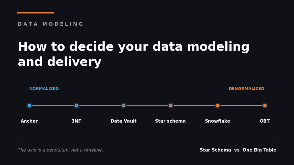
Horizontal data modeling axis, from most normalized (Anchor, 3NF, Data Vault) to most denormalized (Star schema, Snowflake, OBT), in a blue to orange gradient.
I will walk the spectrum from most normalized to most denormalized, and at each stop the question is always the same, what cost was this choice trying to minimize?
3NF and Inmon, write integrity above everything
Third normal form is the leftmost point. Zero redundancy, each fact stored exactly once, everything broken into tables related by key. It is the world of OLTP, of the transactional database. The bottleneck 3NF minimizes is the cost of inconsistent writes. If the customer’s address lives in one place only, you never end up with two diverging addresses. Update one, you updated them all.
Bill Inmon took that philosophy to the data warehouse with the Corporate Information Factory, the top-down approach. You first build a corporate EDW normalized in 3NF, the single source of truth, and only then derive dependent data marts for each area. It is robust and expensive to start. You need to model the whole company before shipping the first dashboard.
The problem with 3NF for analytics is simple. Answering “revenue by category by region last quarter” means joining a dozen tables. In OLTP, that is the price of consistency. In OLAP, it is the main bottleneck.
-- 3NF, each fact stored once, linked by keyCREATE TABLE cidade (cidade_id INT PRIMARY KEY, nome VARCHAR(80), uf CHAR(2));CREATE TABLE cliente (cliente_id INT PRIMARY KEY, nome VARCHAR(120), cidade_id INT REFERENCES cidade(cidade_id));CREATE TABLE pedido (pedido_id INT PRIMARY KEY, data DATE, valor NUMERIC(12,2), cliente_id INT REFERENCES cliente(cliente_id));-- "revenue by state (UF)" requires joining pedido -> cliente -> cidadeSELECT ci.uf, SUM(p.valor)FROM pedido pJOIN cliente c ON c.cliente_id = p.cliente_idJOIN cidade ci ON ci.cidade_id = c.cidade_idGROUP BY ci.uf;
Data Vault, when the source changes every week
One step to the right, with a philosophy of its own. Data Vault was created by Dan Linstedt in the 1990s and formalized as Data Vault 2.0, and it splits the model into three pieces. Starting with hubs (the business keys, insert-only, just the identifier), links (the relationships between hubs, also insert-only and treated as first-class objects) and satellites (the descriptive attributes and their history, versioned via hashdiff).
The genius move is in the links. In a star schema, the relationship lives embedded in the fact table: if you discover that orders now connect to marketing campaigns, you need to alter the fact and backfill. In Data Vault, you just create a new link, link_pedido_campanha, without touching anything that already exists. The model absorbs source changes without breaking.
Which bottleneck does that minimize? The organizational cost of change and audit. The canonical scenario is the company with 30+ source systems, three CRMs from acquisitions, a legacy ERP, event streams, and a new schema landing every week. In pure Kimball, each of those changes blows up ETL and breaks dashboards. In regulated industries (banking, healthcare), Data Vault also gives you full traceability. You can prove where each piece of data came from, when, and from which source.
The cost of Data Vault is Data Vault itself. If you have five source tables and one BI tool, Data Vault only adds complexity with no proportional benefit. And nobody consumes Data Vault directly. It almost always feeds a Kimball or OBT presentation layer on top. It is back-office infrastructure for modeling. The storefront lives elsewhere.
-- Hub, just the business key (insert-only)CREATE TABLE hub_cliente ( hk_cliente BINARY(16) PRIMARY KEY, -- hash of the business key cliente_bk VARCHAR(50), -- natural key from the source load_date TIMESTAMP, record_source VARCHAR(50));-- Link, the relationship as a first-class object (insert-only)CREATE TABLE link_pedido_cliente ( hk_link BINARY(16) PRIMARY KEY, hk_cliente BINARY(16) REFERENCES hub_cliente(hk_cliente), hk_pedido BINARY(16), load_date TIMESTAMP, record_source VARCHAR(50));-- Satellite, attributes + history, versioned by hashdiffCREATE TABLE sat_cliente ( hk_cliente BINARY(16), load_date TIMESTAMP, hashdiff BINARY(16), -- changes whenever any attribute changes nome VARCHAR(120), cidade VARCHAR(80), PRIMARY KEY (hk_cliente, load_date));
Found out orders now link to campaigns? Create link_pedido_campanha and move on with your life. No existing table gets touched.
Anchor modeling, the Swedish cousin that takes normalization to the extreme
If Data Vault is normalized, anchor modeling is normalization pushed to the limit. Created in Sweden by Olle Regardt and Lars Rönnbäck (implementations since ~2004, paper at ER’09), it models everything in sixth normal form with four constructs: anchors (the entity’s identity, a table with basically one column), attributes (each descriptive attribute in its own table, historized if needed), ties (the relationships) and knots (shared, stable values, like marital status or gender).
The principle that sells anchor is: “A big change on the outside becomes a small change on the inside.” Since each attribute is an isolated table, adding a new field never requires an ALTER on a giant entity or a backfill. You just create one more little table. And since everything is historized by design, it handles time (valid time, transaction time) natively.
-- Anchor, just the entity's identityCREATE TABLE CU_Cliente ( CU_ID INT PRIMARY KEY );-- Historized attribute, the name, in a table of its ownCREATE TABLE CU_NOM_Cliente_Nome ( CU_ID INT REFERENCES CU_Cliente(CU_ID), Nome VARCHAR(120), ValidFrom DATE, PRIMARY KEY (CU_ID, ValidFrom));-- Knot, shared and stable valueCREATE TABLE EST_EstadoCivil ( EST_ID INT PRIMARY KEY, EST_Valor VARCHAR(20) );
Which bottleneck does anchor minimize? The same one as Data Vault, cheap structural change and full historization, just more radical. The cost is also higher. Reading anything requires joining dozens of tiny tables (mitigated by table elimination in optimizers that drop unnecessary joins). It is academically beautiful, extremely rare outside niches (insurance, Nordic retail), and almost never the layer the end user touches. Worth knowing to understand how far the “normalized” extreme goes, and why almost nobody lives there.
Star schema and Kimball, the compromise of the expensive-disk era
This is where the heart of the fight lives. Ralph Kimball proposed dimensional modeling. You split the world into fact tables (the metrics, the measurable events, a sale, a click, a payment) and dimension tables (the descriptive context, the customer, the product, the date, the store). Connect everything by keys and you draw a star, the fact in the center, the dimensions around it.
The approach is bottom-up. You deliver one area’s data mart first and stitch the marts together via conformed dimensions (dimensions shared and consistent across areas) and the bus matrix. It solves things that actually matter: Slowly Changing Dimensions (how to track that a customer moved cities without losing history), consistency of definitions across teams, and a structure that mirrors how the business thinks.
Now the part almost nobody talks about. Why does star schema denormalize the dimensions but stop short of OBT? Because it was designed to optimize the logical layer of a row-store database when storage was expensive and scarce. You wanted fewer joins (so you denormalize inside the dimension) but could not afford to repeat the customer’s name across a billion fact rows (so you keep the dimension separate). Star schema is literally the equilibrium point between “joins hurt” and “redundancy is expensive”, calibrated for 1996 hardware.
-- Dimension, denormalized within itself, with a surrogate keyCREATE TABLE dim_cliente ( sk_cliente INT PRIMARY KEY, -- surrogate key (internal to the DW) cliente_bk VARCHAR(50), -- natural key, from the business rule nome VARCHAR(120), cidade VARCHAR(80), uf CHAR(2));-- Fact, metrics + keys to the dimensions (the star)CREATE TABLE fact_pedido ( sk_cliente INT REFERENCES dim_cliente(sk_cliente), sk_data INT, valor NUMERIC(12,2), qtd_itens INT);-- "revenue by state", a single join, against the small dimensionSELECT d.uf, SUM(f.valor)FROM fact_pedido f JOIN dim_cliente d ON d.sk_cliente = f.sk_clienteGROUP BY d.uf;
Slowly Changing Dimensions, the problem star solves and OBT forgets
A quick aside here, because this is where star schema earns its keep and where almost every OBT trips. The customer moved to another city. What do you do with the history? Slowly Changing Dimensions (SCD), from Kimball’s vocabulary, are the strategies for that:
Type 0: never changes. Date of birth, signup date. Frozen.
Type 1: overwrite. You update the city and lose the past. Simple and amnesiac.
Type 2: version. Close the old row, open a new one with valid_from/valid_to and a current flag. History stays intact, and the old fact keeps pointing at the right version of the customer. It is the workhorse.
Type 3: keep only the previous value in an extra column (cidade_anterior). Shallow history, one step back.
Type 4: push the fast-changing attributes into a separate mini-dimension, so the main one does not bloat.
Type 6: a hybrid of 1+2+3 (the name comes from 1+2+3 = 6), combining overwrite, versioning and the previous-value column.
-- dim_cliente with SCD Type 2, every change becomes a new versioned rowCREATE TABLE dim_cliente ( sk_cliente INT PRIMARY KEY, -- changes with each version cliente_bk VARCHAR(50), -- natural key, stable across versions nome VARCHAR(120), cidade VARCHAR(80), valid_from DATE, valid_to DATE, is_current BOOLEAN);
Why does this matter for the Kimball vs OBT debate? Because an OBT that materializes “the current state” and overwrites is doing SCD Type 1 without realizing it, throwing history away. You can do SCD in an OBT (stamping a version on each row), but it is a decision you have to make on purpose. Star schema forces you to face the question “what do I do when it changes?” at modeling time. OBT lets you postpone it until the day someone asks “what city was the customer in on the purchase date?” and the data no longer exists.
Snowflake schema, the normalized dimension (and the name collision)
A variation on star. You normalize the dimensions themselves, breaking, for example, a product dimension into product → subcategory → category → department. It turns into a snowflake. Less redundancy at the cost of more joins. Small irony, the snowflake schema is the philosophical opposite of what the Snowflake warehouse encourages, which is precisely to denormalize hard and let the columnar engine sort it out. Two “snowflakes” pulling in opposite directions on the same architecture diagram.
One Big Table, the era of cheap columnar
The rightmost point. One wide, denormalized table with everything pre-joined. Zero joins at query time. The engine scans and aggregates. It is the modeling that looked like heresy in 2008 and became the default in the modern stack.
-- One Big Table, everything pre-joined once, zero joins at query timeCREATE TABLE obt_pedidos ASSELECT p.pedido_id, p.data, p.valor, c.cliente_id, c.nome AS cliente_nome, ci.nome AS cidade, ci.ufFROM pedido pJOIN cliente c ON c.cliente_id = p.cliente_idJOIN cidade ci ON ci.cidade_id = c.cidade_id;-- "revenue by state" now has no join at allSELECT uf, SUM(valor) FROM obt_pedidos GROUP BY uf;
Why OBT came back, the bottleneck moved from “storage” to “shuffle”
Go back to the Fivetran number, 25% to 50% faster on Redshift, Snowflake and BigQuery. There is no magic in it. It is the physics of today’s hardware.
Observation 1, in a distributed environment, the join is the expensive operation, and the scan is cheap. In a columnar MPP (massively parallel processing) warehouse, data is spread across many nodes. To do a join, the engine often needs a shuffle, moving data over the network between nodes to align the keys before joining. That is very expensive. OBT eliminates the entire join phase, because everything is already on the same row. You swapped the bottleneck. You left CPU/network (join/shuffle) and went to storage/disk (the table is bigger). And storage today is cheap. Compute is what you pay dearly for.
Observation 2, the obvious criticism of OBT already has a technical answer. “But storing the name ‘Johnny Smith-Smithson Johnson Jr. the Third’ repeated a million times is an absurd waste of space!” It would be, in a row-store. In columnar, no. Engines use Run-Length Encoding and dictionary encoding. If the value “Johnny Smith-Smithson Johnson Jr. the Third” appears 1,000 times in a row in a column, storage does not keep the string 1,000 times. It keeps the value and the count. Columnar groups data of the same type, which yields absurdly better compression ratios than row-based, and it only reads the columns the query asked for. The redundancy that gave the 2008 DBA chills is nearly free today. What costs in a columnar warehouse is the access pattern. The stored byte is almost irrelevant.
Observation 3, but star schema did not die, it wins on another axis. OBT wins on raw read speed. Star schema wins on governance and history. Conformed dimensions guarantee that “active customer” means the same thing everywhere, and Slowly Changing Dimensions track change over time in a way OBT, on its own, does not. You do not pick the winner by looking at the query benchmark. You pick it by looking at whether your problem is dashboard latency or consistency of definitions across analysts and areas.
Activity schema, the path that does not fit on the axis
There is a modern approach that rejects the whole axis. The activity schema, created by Ahmed Elsamadisi (founder of Narrator, presented at Coalesce 2021), proposes modeling everything in a single 11-column time-series table, no fact, no dimension, no JSON. Instead of “facts and dimensions”, the data becomes “a customer did an activity at a moment in time”. Each row is an activity: placed an order, visited the site, opened a ticket, canceled.
-- Activity Stream: one row per "entity did activity X at time T"CREATE TABLE activity_stream ( activity_id VARCHAR, -- id of the occurrence ts TIMESTAMP, -- when customer VARCHAR, -- who (the entity) activity VARCHAR, -- what: 'placed_order', 'visited_site'... anonymous_customer_id VARCHAR, feature_1 VARCHAR, -- flexible context per activity feature_2 VARCHAR, feature_3 VARCHAR, revenue_impact NUMERIC, link VARCHAR, activity_occurrence INT, -- 1st, 2nd, 3rd time the entity did this activity_repeated_at TIMESTAMP);
The promise is huge (and the author himself admits it sounds like snake oil). Any business question comes out of that one table, with a single modeling layer whose only dependency is the raw data. “Revenue by month” and “average time to second purchase” come from the same structure, with no new dimensional model built for each question. Where it shines is behavioral and journey analysis, exactly the kind of temporal question (“what did the user do between A and B”) that ties a star schema in knots. The cost is that classic dimension cases (joining an attribute that changes over time) become edge work, solved with special joins like last-before. It is an entire philosophy. It is no single point on the normalization spectrum, and that is why it deserves a spot on the map even though it does not fit on the ruler.
The layer axis, refinement rather than shape
Now the orthogonal axis. Here nobody argues about how much to normalize. The argument is how ready the data is for consumption.
Medallion: bronze, silver, gold
Databricks popularized the term around 2019–2020 along with the lakehouse, but the concept is old and, importantly, it is a logical pattern, with no product attached. You implement medallion on Snowflake, BigQuery, Fabric, whatever you have.
Bronze, ingestion and preservation. Raw data, as close to the source as possible, minimal transformation. Reliable capture, no business rules here.
Silver, cleaning and standardization. Where data becomes usable: dedupe, casts, validation, quarantine of corrupted records, joins that conform entities.
Gold, serving. Aggregated, curated, ready for decisions. This is where you apply Kimball or OBT. Gold is the shape. Medallion is the road to it.
Access usually mirrors trust: bronze restricted to data engineering, silver for scientists and power users, gold open to the broader organization.
Observation 4, medallion’s failure modes are almost always about discipline, almost never about technology. The classics that show up in every engineering post-mortem:
Business rules leaking into bronze (which should be raw).
Silver turning into a “second bronze”, a dumping ground with no governance.
Gold rebuilt from scratch by every team, with no reuse, multiplying divergent definitions.
Getting the three folder names right is the easy part of medallion. The real work is giving each layer a contract and a clear boundary of responsibility. A folder with a pretty name and messy logic is just a lake turning into a swamp with extra steps.
dbt: staging, intermediate, marts
It is the operational version of the same axis, in the analytics engineering world.
Staging, one model per source table, usually materialized as a view. Convention stg___. Here you rename columns, cast, standardize, and that is it. Golden rule: no joins across domains, no aggregation. Why? To preserve the source grain. If you aggregate early, you lock the grain and kill downstream reuse.
Intermediate, int_, where complexity gets absorbed. Joins, business logic stacked in layers. A golden DAG rule: many inputs flowing into an intermediate model is great and expected, many arrows leaving it is a red flag.
Marts, the delivery. fact_/dim_ in Kimball style, or marts by domain (mart_vendas, mart_churn). Materialized as a table, for performance. Each mart represents one entity at a single grain.
Notice that staging→intermediate→marts is exactly bronze→silver→gold with different vocabulary and more opinions about SQL. And that, again, the mart is where shape gets decided. Layer and shape meet in the final product.
The intruder: tidy data is neither star nor OBT
Here comes the concept data scientists (hello, tidyverse community) worship and that the data engineering crowd sometimes does not even know by name.
Hadley Wickham published Tidy Data in 2014 in the Journal of Statistical Software, and defined three rules for “tidy” data: each variable is a column, each observation is a row, each type of observational unit is a table. The mantra that took over the R world and later influenced pandas. It is the analyst’s “normal form”, and it optimizes a very specific bottleneck, the ease of manipulating, modeling and visualizing with vectorized tools. Tidy data goes into a tidy tool and tidy data comes out, and then a small set of operations (melt, split, cast) covers almost any mess.
And here is the tension almost nobody spells out: tidy data is long and narrow, nearly the opposite of OBT, which is wide. The two tribes call opposite things “good modeling”.
Take Wickham’s own classic example, temperature measured in three cities per week. The spreadsheet instinct is one column per city (wide). The tidy version is three columns: week, city, temperature (long). For a ggplot or a seaborn, the long version is trivial to plot. For a BI dashboard listing cities side by side, the wide version is what you want.
The resolution is that neither one is “right”. They serve different layers and purposes. Tidy/long is the consumption shape for statistical analysis and visualization, wide/OBT is the serving shape for BI. A data scientist pulls gold, melts it to get tidy in the notebook, runs the model. There is no contradiction, only translation at the boundaries. The mistake is trying to impose one tribe’s normal form on the other tribe’s layer.
The semantic layer changes the answer again
Just when you think you closed the case with “OBT for reads, star for governance”, a new layer shows up and reshuffles everything, the semantic layer (or metrics layer).
dbt’s own documentation is explicit about this. Without a semantic layer, the recommendation is to denormalize hard in the marts. But if you use the Semantic Layer with MetricFlow, the recommendation flips: stay as normalized as possible, to give the metrics engine maximum flexibility to assemble the joins on the fly.
Why does that happen? Because the semantic layer moves the shape decision to runtime. You define the metric and the entities once, in a normalized and canonical form, and the OBT the BI consumes becomes generated on demand by the query. Star schema stops being the storefront and becomes the input to the semantic layer. Denormalization does not disappear. It just stops being a physical modeling decision and becomes a query compilation decision.
The meta lesson here, which applies to the whole article: every time a new tool changes the economics, the modeling “best practice” changes with it. Columnar reopened OBT. The semantic layer reopened normalization. Whoever treats modeling as dogma is always one hardware generation behind.
Data mart and data mesh: shape meets the organization
So far I have talked about shape and layer. What is missing is the organizational scope axis, which is where data mart and data mesh come in, and where the discussion stops being technical and becomes sociotechnical.
Data mart, the furnished room
A data mart is a slice of the warehouse focused on a domain or department: marketing, finance, logistics. If the warehouse is the house, the mart is the room already furnished for a specific team to live in. In the Kimball tradition (bottom-up), you build the marts first and integrate them via conformed dimensions. In the Inmon tradition (top-down), the corporate EDW comes first and the marts are derived from it. The Kimball vs Inmon fight, deep down, was always about build order and ownership, and never about table shape. Who delivers value first, the business area or corporate?
Data mesh, the mart promoted to an organizational principle
In 2019, Zhamak Dehghani, then at ThoughtWorks, coined data mesh and took that ownership question to its logical extreme. The thesis: the central data team becomes a bottleneck because it lacks domain context, so it builds the wrong thing, and domains wait months for data. The solution is to decentralize, with four principles:
Domain-oriented ownership, whoever generates and understands the data owns it. Marketing owns marketing data. Based on Eric Evans’ domain-driven design.
Data as a product, each domain’s data is treated as a product, with the consumer as the customer, with an SLA, documentation, discoverability. This is the conceptual leap.
Self-serve data platform, a platform that reduces the cognitive load for domains to produce and consume data without reinventing infrastructure.
Federated computational governance, global standards (interoperability, security, contracts) applied in a federated and automated way, with no manual committee.
Data mesh is an operating model, with no table shape attached. But it depends on the shape and layer decisions we just saw. Each domain data product still needs to be modeled (star, OBT, whatever serves), still goes through refinement (medallion/dbt), and still needs a semantic contract to be interoperable. Mesh does not replace modeling. It distributes the responsibility for it.
A warning is in order. Mesh is an organizational change before it is a technical one. Whoever treats it as a pure technology project fails. And plenty of small teams that adopted “mesh” only recreated silos with a fancy name. Mesh solves a problem of organizational scale. If you have one data team and five sources, mesh is overhead, the same way Data Vault is.
Data is no end in itself: modeling is the interface that unblocks everyone
This whole discussion of 3NF, Kimball, OBT, medallion has nothing to do with diagram elegance. It is about who can ask the data a question without opening a ticket.
Think about what happens when modeling is bad. Each business question (“what is the retention of users who came in through campaign X?”) becomes a request to data engineering. Engineering goes into a queue. The analyst waits three days, gets a number, discovers it was the wrong metric, files the request again. The data scientist trusts no table and rebuilds the whole pipeline in their own notebook, creating the company’s 14th definition of “active user”. Data became an end in itself, an asset the company collects, stores, and extracts a ridiculous fraction of value from, because the human bottleneck is the data team.
Now think about the opposite. When modeling is good, it is the API. The well-defined grain, the consistent names, the conformed dimensions, the semantic layer with canonical metrics, all of that is the contract that lets the analyst, the scientist and the business folks explore on their own. The preserved grain of a stg_orders is what allows three different questions to be answered without rewriting anything. The gold layer opened up with governance is what gets engineering out of the way. Mesh’s “data as a product” is literally that: data treated as a product that documents itself and serves itself.
That is the reading that holds the whole article together. Good physical modeling is what lets the database scale without betraying you in production. Good metric modeling is what lets the experiment be trustworthy and fast. Good analytical modeling is what lets the whole company ask questions. The common thread is always the same, good modeling is the kind that gets out of people’s way.
That is the final criterion, and it beats any benchmark. Do not ask “is this modeling Kimball or OBT?”. Ask “after this modeling, how many more people can answer their own question without asking me for permission?”. If the answer is “more”, you got it right, whatever the name on the diagram.
Recommendations off the top of my head
What I actually take from this study, in order of importance.
Pick the point on the axis by the bottleneck. Cheap storage and read-dominated workloads? OBT in gold solves it and beats star schema on the benchmark. Governance, history and consistency across many teams? Star schema with conformed dimensions and SCD. Thirty sources changing every quarter and regulatory audits? Data Vault in raw, Kimball or OBT in presentation. Five sources and one BI tool? Simple star schema.
Do not confuse shape with layer. “We use medallion” and “we use Kimball” do not compete, they compose. Shape is decided in gold/mart. Bronze/silver/gold is the road there. Whoever says they replaced one with the other is measuring kilometers in kilograms.
Star schema at the input of the semantic layer, OBT in gold for direct consumption. If you have a metrics layer, keep it normalized and let the layer generate the wide table at query time. If you do not, denormalize hard in the mart. The tool defines the answer, never the dogma.
Tidy in the notebook, wide in the dashboard. Do not impose the data scientist’s long format on the BI layer, nor the wide OBT inside the statistical modeling pipeline. Translate at the boundaries, it is cheap.
Data Vault, anchor and data mesh only when you have their problem. All three are answers to problems of scale (of sources, of structural change, of organization). Anchor takes it to 6NF and rarely leaves its niches. Applied in a small environment, they become pure overhead that rots fast. The adoption cost is real and charged every day.
Measure before you denormalize. Before dumping everything into an OBT, look at the real query pattern (which join hurts, which column gets filtered, what the volume is). Speculative denormalization is optimizing in the dark. It looks like a gain and usually turns out to be fragmentation and maintenance cost.
Treat modeling as a product, with the diagram as a byproduct. The success of your modeling is measured in people unblocked. Reaching third normal form earns you nothing on its own. Document the grain, expose the metric definition, give governed access to gold. Modeling is the company’s self-service interface to its own data.
If your question is behavioral, consider the activity schema before torturing a star. “What did the user do between signup and first purchase”, “how long until they come back”, funnel and journey are temporal questions that tie fact/dimension in knots and come out naturally from an activity stream. You do not need to adopt Narrator’s whole stack to steal the event model idea.
Conclusion
Anchor, 3NF, Data Vault, star schema, snowflake schema and OBT are the same axis, normalization versus denormalization, and each one is a point calibrated for one era’s bottleneck. Star schema is the right answer to a 1996 economics question, and columnar changed the question. Activity schema does not even enter the axis. It rejects fact/dimension and models the world as a sequence of events. Bronze/silver/gold and staging/intermediate/marts are another axis, refinement, and they compose with the first instead of competing. Tidy data is the analyst’s normal form, long where OBT is wide, and the tension between them vanishes once you understand they serve different layers. Data mart and data mesh lift the discussion to the organizational plane, where the question becomes who owns the data and how governance gets run.
The point that cuts through all of it is that data infrastructure rarely has an absolute answer. It has an answer conditional on your bottleneck and on the economics of your stack. Modeling is economics, ergonomics and lower cognitive load, with aesthetics nowhere in it, and in the end it is the question of who you are trying to unblock. Treated as dogma, it is always one hardware generation behind.
The right question was never “Kimball or OBT”. It was “where is my bottleneck, and who needs to explore this data without asking me for permission”.
A good data model is never the prettiest one on the diagram. It is the one that gets out of people’s way and lets them ask.
Kimball, R., Ross, M. (2013). The Data Warehouse Toolkit: The Definitive Guide to Dimensional Modeling. 3rd ed. Wiley.
Inmon, W. H. Building the Data Warehouse / Corporate Information Factory (CIF).
Linstedt, D., Olschimke, M. (2015). Building a Scalable Data Warehouse with Data Vault 2.0. Morgan Kaufmann.
Dehghani, Z. (2022). Data Mesh: Delivering Data-Driven Value at Scale. O’Reilly. (Concept coined in 2019 at ThoughtWorks; four principles: domain ownership, data as a product, self-serve data platform, federated computational governance.)
Regardt, O., Rönnbäck, L., Bergholtz, M., Johannesson, P., Wohed, P. (2009). “Anchor Modeling — An Agile Modeling Technique Using the Sixth Normal Form for Structurally and Temporally Evolving Data”. ER’09. https://www.anchormodeling.com
Elsamadisi, A. (2021). “Introducing the activity schema: data modeling with a single table”. Coalesce / dbt. https://www.activityschema.com